Customer Segmentation RFM

#mysql #cloud #tableau #personal

Goals and Takeaway

Project Goal: My goal was to apply my knowledge of MySQL in a practical setting. I wanted to strengthen my ability to extract behavioural patterns from transactional data and translate those into actionable segmentation.

Key Takeaways: In this project, I deepened my ability to use SQL for behaviour-driven customer segmentation and learned how to define and tune thresholds that reflect customer value. I also got more comfortable structuring layered queries using CTEs and CASE logic. I realized how even simple metrics, when combined thoughtfully, can unlock nuanced decision-making.

Environment

• Cloud Database - Creating an RDS instance in AWS
• Tableau

Sources

• Data and overall project structure: RFM-Based-Customer-Segmentation.
• RFM segmentation by Optimove

Background

The client, a sticker company serving retail partners, is seeking an analysis of customer purchasing behaviour to support targeted marketing efforts aimed at increasing loyalty, improving retention, and driving revenue growth. To enhance newsletter campaign effectiveness, the analysis will also include a business performance overview and insights into peak customer activity by time of day. The dataset spans the period from December 2010 to December 2011.

Data Cleaning

Creating a new table to edit from

CREATE TABLE table_retail_
LIKE tableRetail;

INSERT table_retail_
SELECT *
FROM tableRetail;

From string to date time

UPDATE table_retail_
SET InvoiceDate = STR_TO_DATE(InvoiceDate, '%c/%e/%Y %H:%i');

ALTER TABLE table_retail_
MODIFY InvoiceDate DATETIME;

Finding and removing duplicates

Determining the number of duplicates

WITH duplicates AS
(
SELECT *,
ROW_NUMBER() OVER(
PARTITION BY Invoice, StockCode, Quantity, InvoiceDate, Price, Customer_ID, Country) AS row_num
FROM table_retail_
)
SELECT COUNT(*) AS row_count
FROM duplicates
WHERE row_num > 1
;

Output: 260

Removing duplicates

I proceeded by creating another table (Table_Retail_1).

• This table has the extra rows that I want to delete.
• I can then delete the data when the row_num is >1.

DELETE
FROM Table_Retail_1
WHERE row_num > 1;

Removing missing or erroneous data

SELECT * 
FROM Table_Retail_1
WHERE Price IS NULL
OR Price = ''
OR Price = '0';

Output

DELETE
FROM Table_Retail_1
WHERE Price = '0';

Analysis

Executive Summary

Between December 2010 and 2011, the stakeholder generated £254,172 in revenue within the UK. This was driven by 716 orders placed by 110 customers, yielding an average order value of £20.18.

The top 10 most lucrative products contributed between £2,000 and £9,000 in revenue each. In terms of sales volume, the top 10 best selling products saw between 1,500 and 7,700 units sold. Comparatively, around 25% of all listed products were purchased only once during this period, indicating potential stagnation.

Sales peaked the most between August and December. Totalling 60% of the total revenue, this period marks the business’s most lucrative stretch. When examining time-of-day patterns, the majority of purchases occurred in the afternoon (66%), followed by morning transactions (30%) and evening sales represented only 4% of total activity. This trend aligns with most of the customers operating business hours.

The customer segmentation analysis highlights that nearly one-third of clients are loyal or top-tier, while another third requires renewed engagement to avoid churn. Potential loyalists (21%) represent a growth opportunity with strategic nurturing. Dormant and lost customers make up 17%, pointing to areas for reactivation or letting go.

Looking forward, a more granular customer segmentation analysis will help uncover deeper loyalty dynamics and inform tailored retention strategies for all segments. To that effect, a few questions have been drawn out and addressed as a starting point.

Performance overview

Between December 2010 and 2011, the stakeholder generated £254,172 in revenue within the UK. This was driven by 716 orders placed by 110 customers, yielding an average order value of £20.18.

SELECT
	DISTINCT Country							AS country,
	COUNT(DISTINCT Customer_ID)					AS nb_of_customers,
    COUNT(DISTINCT Invoice)						AS nb_of_orders,
    ROUND(AVG(Price * Quantity),2)  			AS avg_purchase_amount,
    FORMAT(ROUND(SUM(Price * Quantity)))	    AS total_revenue
FROM Table_Retail_1
GROUP BY Country;

Output

Products performances

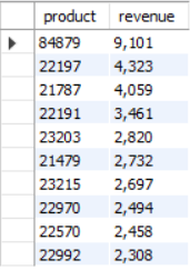
The top 10 revenue-generating products each delivered between £2,000 and £9,000. Notably, product #84879 generated £9,101, more than double that of product #22197 (the second highest earner at £4,323).

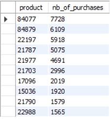
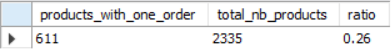
In terms of sales volume, the 10 best-selling products sold between 1,500 and 7,700 units each. On the other end of the spectrum, approximately 25% of the inventory sold only one unit, representing 611 potentially stagnant products in need of review or repositioning.

Products that brought the most revenue

SELECT 
	StockCode								AS product,
    FORMAT(ROUND(SUM(Price * Quantity)),0) 	AS revenue
FROM Table_Retail_1
GROUP BY product
ORDER BY SUM(Price * Quantity) DESC
LIMIT 10;

Output

Best selling products

SELECT 
	StockCode						AS product,
    SUM(Quantity)					AS nb_of_purchases
FROM Table_Retail_1
GROUP BY product
ORDER BY nb_of_purchases DESC
LIMIT 10;

Output

Products ordered once

SELECT 
	COUNT(*) AS products_with_one_order,
     total.total_nb_products,
    ROUND(COUNT(*) * 1.0 / total.total_nb_products, 2) AS ratio
FROM (
  SELECT StockCode
  FROM Table_Retail_1
  GROUP BY StockCode
  HAVING COUNT(DISTINCT Invoice) = 1
) AS one_order_products,

(
  SELECT COUNT(DISTINCT StockCode) AS total_nb_products
  FROM Table_Retail_1
) AS total;

Output

Purchases and revenues per interval

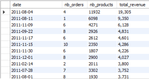
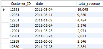
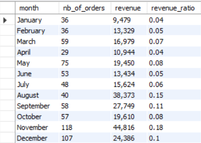
Between December 2010 and December 2011, daily purchases peaked from August through November, accounting for 60% of total revenue during the year. August and November were the most profitable months, contributing respectively 15% and 18% of annual revenue. Standout sales days included November 4th (£19,305) and November 11th (£9,350), both driven by customer #12931, making them the most lucrative dates of the period.

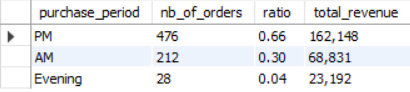
Analysis of purchasing habits reveals a strong afternoon preference from the clients: 66% of all orders occurred in pm, followed by 30% in the morning. Evening purchases were minimal, representing just 4% of overall activity.

Daily

SELECT 
	DISTINCT DATE(InvoiceDate)					AS `date`,
    COUNT(DISTINCT Invoice)						AS nb_orders,
    SUM(Quantity)								AS nb_products,
    FORMAT(ROUND(SUM(Price * Quantity)),0)	    AS total_revenue
FROM Table_Retail_1
GROUP BY 1
ORDER BY SUM(Price * Quantity) DESC;

Output Sample

Highest paying customers per interval

SELECT 
	DISTINCT Customer_ID,
    DATE(InvoiceDate)                               AS `date`,
	FORMAT(ROUND(SUM(Price * Quantity)),0)			AS total_revenue
FROM Table_Retail_1
GROUP BY 1,2
ORDER BY SUM(Price * Quantity) DESC;

Output sample

Monthly

WITH monthly_data AS
(
SELECT
Invoice,
InvoiceDate,
Price * Quantity AS total,
MONTH(InvoiceDate) AS month_num,
    CASE 
		WHEN MONTH(InvoiceDate) = 1 THEN 'January'
        WHEN MONTH(InvoiceDate) = 2 THEN 'February'
        WHEN MONTH(InvoiceDate) = 3 THEN 'March'
        WHEN MONTH(InvoiceDate) = 4 THEN 'April'
		WHEN MONTH(InvoiceDate) = 5 THEN 'May'
        WHEN MONTH(InvoiceDate) = 6 THEN 'June'
        WHEN MONTH(InvoiceDate) = 7 THEN 'July'
        WHEN MONTH(InvoiceDate) = 8 THEN 'August'
		WHEN MONTH(InvoiceDate) = 9 THEN 'September'
        WHEN MONTH(InvoiceDate) = 10 THEN 'October'
        WHEN MONTH(InvoiceDate) = 11 THEN 'November'
        ELSE 'December'
    END AS month
  FROM Table_Retail_1
  ),
total_revenue AS 
(
SELECT SUM(total) AS grand_total FROM monthly_data
)

SELECT month,
COUNT(DISTINCT Invoice)  AS nb_of_orders,
FORMAT(ROUND(SUM(total)),0) AS revenue,
ROUND(SUM(total) / (SELECT grand_total FROM total_revenue),2) AS revenue_ratio
FROM monthly_data
GROUP BY month_num;

Output

Per time of day

SELECT 
purchase_period,
COUNT(DISTINCT Invoice)  AS nb_of_orders,

ROUND(
COUNT(DISTINCT Invoice) / 
    (SELECT COUNT(DISTINCT Invoice) FROM Table_Retail_1),
    2
  ) AS ratio,
  
FORMAT(ROUND(SUM(total)), 0) AS total_revenue
FROM 
(
SELECT
Invoice,
Price * Quantity AS total,
    CASE 
      WHEN TIME(InvoiceDate) BETWEEN '00:00:00' AND '11:59:59' THEN 'AM'
      WHEN TIME(InvoiceDate) BETWEEN '12:00:00' AND '17:59:59' THEN 'PM'
      ELSE 'Evening'
    END AS purchase_period
  FROM Table_Retail_1
) AS sub

GROUP BY purchase_period
ORDER BY ratio DESC;

Output

Customers

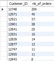
Customer #12748 stands out as a clear outlier, having placed 209 orders, roughly four times more than the next most active customer, #12971.

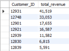
Interestingly, customer #12931 surpasses #12748 in total revenue, generating £41,519 across just 15 transactions, compared to #12748’s £33,053. This highlights customer #12931’s significantly higher average order value and positions them as a key high-value client.

Customers with the most orders

SELECT 
	DISTINCT Customer_ID,
	COUNT(DISTINCT Invoice)					AS nb_of_orders
FROM Table_Retail_1
GROUP BY 1
ORDER BY nb_of_orders DESC;

Output Sample

The highest paying customers

SELECT 
	DISTINCT Customer_ID,
	FORMAT(ROUND(SUM(Price * Quantity)))		AS total_revenue
FROM Table_Retail_1
GROUP BY 1
ORDER BY SUM(Price * Quantity) DESC;

Output Sample

RFM customer segmentation

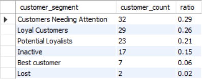
Customer segmentation reveals that loyal and best customers account for about 30% of the total clientele. Interestingly, about the same proportion applies to the “customers needing attention” segment. Potential loyalists make up 21% of the customer base and show promising potential to evolve into high-value clients with the right nurturing. Meanwhile, 15% of customers have remained dormant for an extended period, and 2% are classified as lost.

As part of a deeper customer segmentation and tailored retention strategy, a set of preliminary questions have been outlined and addressed to guide future analysis.

Box plots

These absolute thresholds have been determined by referring to box plots data distribution. Removing the outliers helped determine an optimal range to classify the number of purchases and revenues generated per customer. These thresholds have been established in concurrence with the current clientele’s habits and can be customized to the stakeholder’s desire.

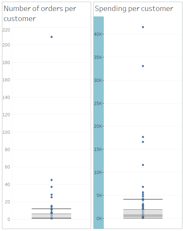
Number of orders per customer

This plot showcases the following:

• Upper whisker: 12
• Upper hinge: 6
• Median: 2
• Lower hinge: 1
• Lower whisker: 1

Spending per customer

This plot showcases the following:

• Upper whisker: 4091
• Upper hinge: 1857
• Median: 849.5
• Lower hinge: 354
• Lower whisker: 38

RFM query

CREATE TABLE rfm_segm_ AS
WITH rfm_base AS(
    SELECT   customer_id									AS customer_id,
             MAX(invoicedate)								AS last_order_date,
             COUNT(DISTINCT invoice)						AS order_count,
             SUM(price * quantity)							AS total_price
      FROM   Table_Retail_1
  GROUP BY   customer_id
),

rfm AS(
    SELECT 		customer_id									AS customer_id,
				DATEDIFF('2011-12-31', last_order_date)	 	AS recency,
				order_count									AS order_count,
				total_price									AS total_price
      FROM   rfm_base
),

customer_segment_base AS (
  SELECT 
		customer_id,
         CASE
           WHEN recency <= 30 THEN 5
           WHEN recency <= 60 THEN 4
           WHEN recency <= 120 THEN 3
           WHEN recency <= 180 THEN 2
           ELSE 1
         END AS recency,
         CASE
           WHEN order_count = 1 THEN 1
           WHEN order_count <= 2 THEN 2
           WHEN order_count <= 3 THEN 3
           WHEN order_count <= 6 THEN 4
           ELSE 5
         END AS frequency,
          CASE
           WHEN total_price <= 100 THEN 1
           WHEN total_price <= 500 THEN 2
           WHEN total_price <= 1000 THEN 3
           WHEN total_price <= 2000 THEN 4
           ELSE 5
         END AS monetary
  FROM rfm
  )

  SELECT   customer_id,
           recency,
           frequency,
           monetary,
           CASE WHEN (recency + frequency + monetary) = 15             THEN 'Best customer'
                WHEN (recency + frequency + monetary) >= 12            THEN 'Loyal Customers'
                WHEN (recency + frequency + monetary) BETWEEN 9 AND 11 THEN 'Potential Loyalists'
                WHEN (recency + frequency + monetary) BETWEEN 6 AND 8  THEN 'Customers Needing Attention'
                WHEN (recency + frequency + monetary) BETWEEN 4 AND 5  THEN 'Inactive'
                WHEN (recency + frequency + monetary) <= 3             THEN 'Lost'
           END AS customer_segment
     FROM  customer_segment_base
 ORDER BY  recency DESC,
           frequency DESC,
           monetary DESC;

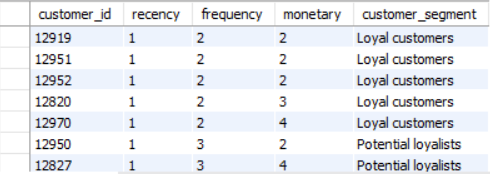
Output sample

RFM ratio

SELECT 
customer_segment,
COUNT(customer_id)  AS customer_count,

ROUND(
COUNT(customer_segment) / 
    (SELECT COUNT(customer_segment) FROM rfm_segm),
    2
  ) AS ratio
  
  FROM rfm_segm_
GROUP BY customer_segment
ORDER BY ratio DESC;

Output

Preliminary questions

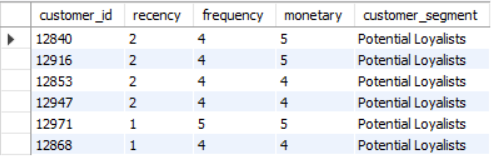
Who were frequent high paying customers and have been inactive in the last 6 months?

SELECT *
FROM rfm_segm
WHERE recency <= 2
AND frequency >= 4
AND monetary >= 4;

Output

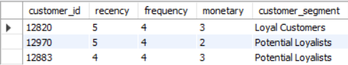
Which active customers could increase their purchase amounts?

SELECT *
FROM rfm_segm
WHERE recency >= 4
AND frequency >= 4
AND monetary <= 3;

Output

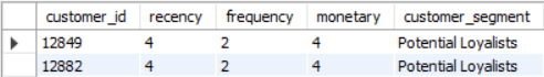
Who are the new high paying customers?

SELECT *
FROM rfm_segm
WHERE recency >= 4
AND frequency = 2
AND monetary >= 4;

Output

Clarifying Questions

Defining the next steps of the analysis

• Would the stakeholder like to include product category data in the next steps to enhance insights into purchase behaviour and support more targeted engagement strategies?
• Which customers or purchase behaviours would the marketing team want to explore more?
• Would a granular segmentation of customers needing attention be useful in extracting purchase patterns and separating subgroups belonging to this broad category?

Assumption and caveats

More than 365 days of data

• The data frame spans from December 1st, 2010 to December 9th, 2011. While this additional week slightly extends the one-year window, its impact on the overall accuracy of the extracted insights is minimal.